Method
New Methods for Solving the Criminological Puzzle
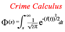
The solution to the criminological puzzle requires some new methods of working with the problem. For instance, a solution to the bivariate probit model of propensity, sanctioning, and crime with multiple time varying covariates requires calculus, because the formula for crime is an integral function derived from the intersection of propensity and sanctioning. For most problems, we will need to solve for z, which presents challenges. One simplification of the process is to use the method of probits. The time varying components do not fit any standard mathematical functions. The developmental curves are complex, and the short and medium term intra-individual variation are the result of multiple random and chaotic processes. These problems are more manageable if some new ways of approaching the problem are developed. The following discussions will focus on three innovations in the process of model building in criminology, 1) crime calculus, 2) solving for z, 3) the method of probits, 4) model fitting and developmental trajectory modeling in Excel, and 5) working with variation.

Method #1: Crime Calculus
An understanding of crime requires an edge centered view of the world, which is different from the traditional mean centered view. The majority of people are not committing serious crimes on a daily basis, but they have a nonzero probability of committing a crime. The average person’s criminal propensity is also fluctuating over time, sometimes remaining relatively stable and sometimes making huge transitions in a short period. When examining an entire population of individuals with fluctuating criminal propensities, calculus is required in order to determine how changes in propensity and sanctioning levels produce variation in crime rates.

Method #2: Solving for z, μ, & σ
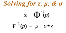
Crime rates can be interpreted as the probability of crime, given some unknown criminal propensity distribution and sanctioning level. If criminal propensity is normal, and sanctioning is asymmetric, it is possible to use the crime rate to estimate the mean (μ) and standard deviation (σ) of the criminal propensity distribution. The process involves converting the probability of crime (p) into a z score using the “probit” or “basic quantile function” [Φ-1(p)] which is the inverse of the standard normal distribution function. The z scores can be used to estimate the mean (μ) and standard deviation (σ) of the criminal propensity distribution using the general quantile function [F-1(p)= μ + σ*Φ-1(p)].

Method #3: The Method of Probits
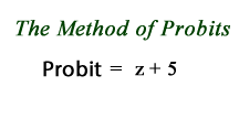
In theory, the z scores generated from crime rates can vary from negative to positive infinity. In practice, the z scores rarely vary beyond a negative to positive five. The negative z scores are hard to work with, and so the method of probits involves adding five to the z scores. This creates a distribution of probit scores that ranges from 0-10. The method of probits facilitates the visualization of time varying criminal propensity distributions.

Method #4: Model Fitting
In order to solve problems like the age crime curve, multiple models need to fit together in a precise manner. Traditional methods of statistical null hypothesis testing do not work in this context. It is necessary to first fit these models together manually in programs like Excel. There are several unrelated mathematical processes at work, and when each of these processes is accounted for in the model, the solution emerges.

Method #5: Working With Variation
Traditional methods of modeling traits focus on the stability of behavior. Newer trait models focus on traits as combinations of states. Researchers are beginning to realize that people’s tendencies to act in a certain way have large short term fluctuations. Traditional models treat this short term fluctuation as “error.” The error model does not reflect reality. Although it is difficult to deal with fluctuation, it is important to develop new methods of studying fluctuations in behavior in order to understand the processes involved.
