Crime Calculus
Crime Calculus
Crimes are random events that occur under the proper conditions. Crimes occur when a person with a sufficiently high criminal propensity crosses the line and behaves in a way that is considered to be sufficiently harmful so that the society that the person is in will sanction the behavior. In order to model crime rate creation at the population level, calculus is needed. Fortunately, much of the work needed to develop a crime calculus has been done by microbiologists. This work simply needs to be adapted to the study of crime.

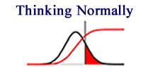
Thinking Normally
One of the skills that is needed when working with a crime calculus is the ability to think normally. The relationship between criminal propensity, sanctioning, and crime rates is non-linear. Because, criminal propensity is normally distributed and the sanctioning process is highly asymmetric, the crime rates follow a sigmoid curve with changes in propensity or sanctioning. For example, if one assumes that the criminal propensity distribution is standard normal, and z ranges from 5 to +5, it takes a 29% increase in criminal propensity to create a 5% jump in the crime rate from 1% to 6%. However, it only takes a 2.6% change in propensity to get the crime rate to rise 5% from 45% to 50%. If criminologists are going to deal with the non-linear nature of the relationship between criminal propensity and crime, they need to study the calculus behind normal distributions, asymmetric selection, and non-linear accumulation over time.

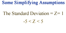
Some Simplifying Assumptions
The math for the normal distribution is rather messy, and it will help initially to make some simplifying assumptions. The first assumption is that the standard deviation of the normal distribution = Z = 1. The second assumption is that Z varies from -5 to 5. Although neither of these assumptions is necessarily true, these assumptions do provide a basis for some initial modeling. These assumptions will have to be revisited later to see if they are relatively accurate.

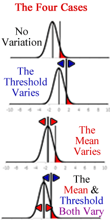
The Four Cases
In order to study both criminal propensity and sanctioning, it is important to determine what is varying. If the standard deviation of the normal distribution is set to one, then there are four possible cases that represent possible types of variation in the mean and threshold level. The first case is no variation in mean propensity or the sanctioning threshold. This happens most of the time in a single community, where crime rates remain fairly constant over time. The second case occurs when there is variation in the sanctioning threshold, but criminal propensity is constant. This occurs when there is a change in the legal system which affects the apparent crime rate. The third case occurs when there is variation in the mean level of criminal propensity, but not in the sanctioning threshold. The second case occurs in the age crime curve. Finally, the last case is where criminal propensity and the sanctioning threshold are both changing. This is often the case in comparative criminology, where the criminologist is interested in differences in crime rates between communities. In this case, it is hard to determine why crime rates are varying. These four cases are important for the analysis of the relationship between criminal propensity, sanctioning, and crime rates.

What Do Germs and Criminals Have In Common?
The basis for a crime calculus has already been developed by microbiologists. Microbiologists have dealt with normally distributed populations in the presence of asymmetric selection processes for some time. This problem is routine when trying to estimate germ kill rates in the presence of antiseptics. Germ kill rates almost invariably follow a sigmoid response curve as the antiseptic strength increases. This is essentially the same process that occurs with crime rates. Brooks (1918) was the first to develop the calculus underlying this process. He demonstrated that the accumulation process generating the germ kill rates can be modeled as an integral using the cumulative distribution function (CDF) for the underlying probability distribution function (PDF).

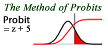
The Method of Probits
One way to simplify the process of working with normal distributions is to use the method of probits. The method of probits was developed by Bliss (1934; 1935) in order to simplify the process of translating germ kill rates to antiseptic strengths. The method of probits is simply a mathematical transformation that simplifies working with normal distributions, z-scores, and rate plots. the method of probits involves taking the crime rate, converting the value to a z-score using an inverse normal distribution function, and adding five to the result. The probits tend to range from 0-10, and make the process of working with nonlinear crime rates a little easier.
